Black-box Testing

Black-box tests are derived from a specification or another description of externally observable behavior without relying on the internal implementation of the test object. Black-box techniques can be used for both functional and non-functional testing. For non-functional testing, the ISO/IEC 25010 product quality model provides a useful classification of quality characteristics.

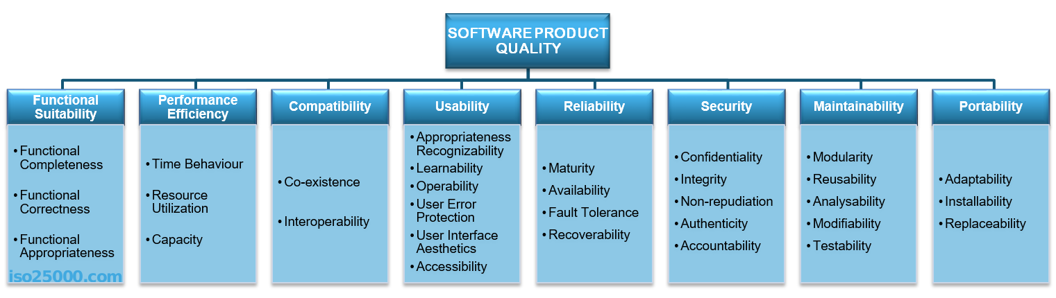
Common black-box techniques covered in this chapter include:

• Equivalence partitioning
• Boundary value analysis
• Decision table-based testing
• State transition testing
• Use case-based testing

Equivalence partitioning

During equivalence partitioning, data are divided into partitions whose members are expected to be processed in the same way by the test object.

• A representative value may be selected from each partition because the values in that partition are expected to be treated equivalently. More than one representative may still be justified by risk or uncertainty.
• For one particular partitioning of an input or output domain, the partitions should be disjoint and together cover the relevant domain.
• An invalid partition contains values that the test object should reject or handle as invalid. When several invalid conditions exist, they are usually tested separately so that one failure does not mask another.
• Partitioning can be refined.

Partitions can be derived from input values, expected outputs, time-related values, interface parameters, configuration values, or other testable characteristics.

Error message should be provided

When testing invalid partitions, the program should provide some kind of error message.

EP example

As an example, consider the following program that expects an integer as input. The program returns a correct result if the input is positive and less than 10,000, or negative and greater than -10,000. During equivalence partitioning, valid input data are divided into two classes: the valid positive and the valid negative partition. Invalid input data are divided into three classes: the invalid positive, the invalid negative partition, and the singleton set containing zero.

Equivalence partition	Values
Valid positive	1 to 9999
Valid negative	-9999 to -1
Invalid positive	10000, 10001, ...
Invalid negative	-10000, -10001, ...
Invalid zero	0

Boundary value analysis

Boundary value analysis (BVA) is a technique based on testing the boundaries of equivalence partitions. Therefore, it can only be applied to ordered partitions. The minimum and maximum values of a partition are the boundary values. In boundary value analysis, if two elements belong to the same partition, every element between them must also belong to the same partition.

• Errors often occur at edge cases.
• These are often linked to characteristic program structures (e.g., branches). Examples include swapping relations, or starting a loop from the wrong index.
• We use it together with equivalence partitioning.
• It can be two-valued or three-valued.
• For boundary tests, the smallest distance between neighboring elements must be known (precision specified).

Two-point boundary value analysis

In two-point boundary value analysis, each boundary has two coverage elements: the boundary itself and the nearest neighbor belonging to the adjacent partition. To achieve 100% coverage with two-point boundary analysis, the test cases must test every coverage element, i.e., every identified boundary. Coverage is defined as the ratio of the number of tested boundary values to the total number of identified boundary values, expressed as a percentage.

Three-point boundary value analysis

In three-point boundary value analysis, each boundary has three coverage elements: the boundary itself and both of its neighbors. Therefore, in three-point boundary analysis, some coverage elements may not be boundary values. To achieve 100% coverage with three-point boundary analysis, test cases must test every coverage element, i.e., every identified boundary and its neighbors. Coverage is defined as the ratio of the number of tested boundary values and neighbors to the total number of identified boundary values and neighbors, expressed as a percentage.

Two-point and three-point boundary value analysis

Three-point boundary value analysis is stricter than two-point, as it can find errors that two-point boundary value analysis misses. For example, if the statement if(x ≤ 10)... is incorrectly implemented as if (x = 10)..., test data derived from two-point boundary analysis (x = 10, x = 11) will not find the error. However, x = 9 derived from three-point boundary analysis likely will.

Example

Suppose we have a function that accepts a positive integer as a parameter, and if it is less than 100 it calls function A, otherwise it calls function B. In this example, the function input can be divided into two valid partitions. In one case [1,2,...,99], the other partition is [100, 101,...]. Our boundary is 100, and in the two-valued check, the first test case will be 99 from the first partition, while 100 from the second. However, we also have an invalid partition: zero and negative numbers. Around 0 we use three-point analysis, so the test cases can be -1, 0, and 1.

Test cases for the previous example

In the previous example, a three-point test for the valid partition can be: 99, 100, 101.

Decision table-based testing

Decision tables are used to test the implementation of system requirements that determine how different combinations of conditions produce different outputs. Decision tables can be effectively used to capture complex logic, e.g., business rules.

When creating a decision table, input data are organized into a table in which columns represent test cases, while rows contain the conditions associated with the test cases. The cells contain the specific test conditions for the test case. The table also includes an operations block, whose rows are the possible operations, while their intersection with the test cases contains the operations derived for that test case from the specific values of the test conditions.

A limited-entry decision table represents conditions and actions using binary values, supplemented by a notation for conditions that do not affect a particular rule.

In the conditions block:

• T (True) indicates that the condition is satisfied.
• F (False) indicates that the condition is not satisfied.
• – means that the condition’s truth value is irrelevant to the outcome of that particular rule (a “don’t care” value).
• An infeasible combination should be omitted or explicitly marked as infeasible. Feasibility applies to the complete combination of conditions in a rule column, not to a single condition row in isolation.

In the operations block:

• X indicates that the operation must be executed under the given set of conditions.
• A blank cell indicates that the action is not performed for that rule.

A complete decision table represents every feasible combination of conditions. It can be simplified by omitting infeasible combinations and minimized by merging rules that produce the same actions when one or more conditions are irrelevant.

Ticketing System

Consider an airline ticketing system whose discount calculation must be tested. The following business rules must be verified:

• If the passenger is under two years old and travels within the state, they get an 80% discount.
• If the passenger is under two years old and travels on an international flight, the discount is 70%.
• Passengers aged 2–16 receive a 10% discount, but if they have an early booking, they get a 20% discount.
• Frequent flyers get a 15% discount, except in the case of early booking, in which case they also get a 20% discount.
• On international flights, traveling in off-season grants a 15% discount.

If multiple conditions are met, the passenger gets the larger discount. If the discount is the same, then either case can be chosen as appropriate.

The following minimized table illustrates the rules that produce a discount. It is not a complete table for all passengers because combinations producing no discount are not shown.

Conditions	1	2	3	4	5	6	7
Under 2 years	T	T	F	F	–	–	–
2–16 years	F	F	T	T	–	–	–
Frequent flyer	–	–	F	–	T	T	–
Intra-state flight	T	F	–	–	–	–	F
Early booking	–	–	F	T	F	T	–
Off-season	–	–	F	–	–	–	T
Actions
10% discount			X
15% discount					X		X
20% discount				X		X
70% discount		X
80% discount	X

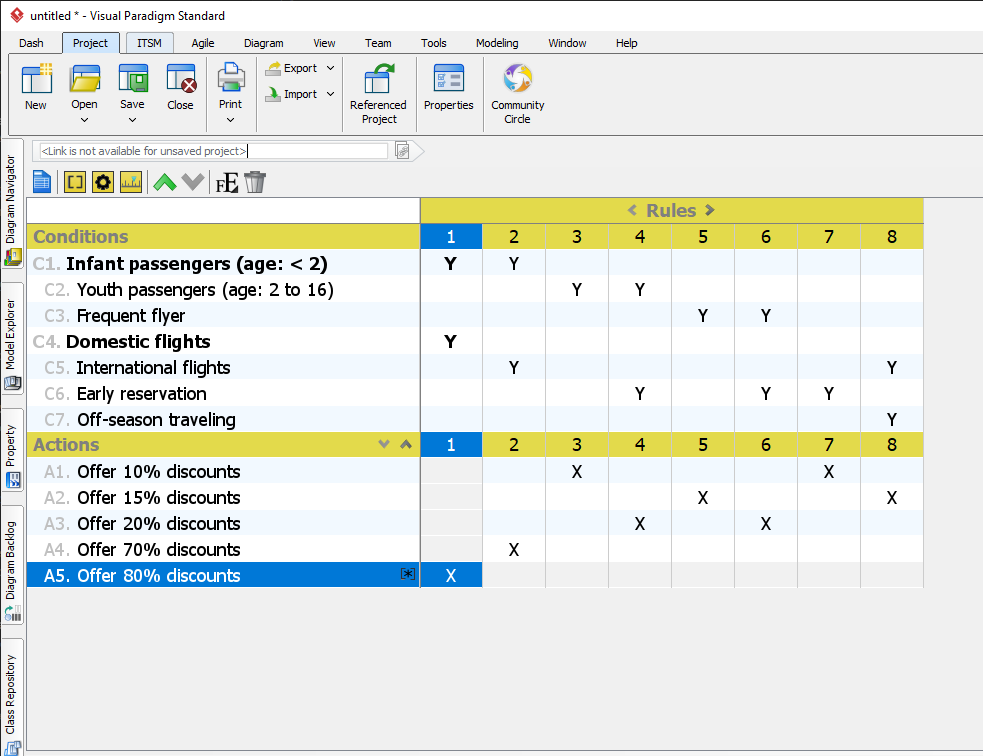
Decision tables can also be created in spreadsheet and word-processing applications. Dedicated modelling tools, such as Visual Paradigm, support this representation. The following figure shows the table in such a tool:

State transition testing

State transition testing is a black-box testing technique in which changes in input conditions cause state changes or output changes in the application under test (AUT). This method helps analyze the behavior of the application under different input conditions and ensures that all possible system responses to valid and invalid transitions are verified.

In state transition testing, we describe the system using a state-transition model, where the system is represented as a finite-state machine. The transitions connecting the states are considered executable test steps. The model has four main components:

• States: The distinct, stable situations of the software (e.g., Open, Closed, Locked).
• Transitions: The changes from one state to another, typically caused by input or internal events.
• Events (or inputs): The triggers that cause a transition to occur (e.g., close file, enter password).
• Actions or outputs: The activities or outputs produced as a result of a transition (e.g., displaying an error message).

The mathematical foundations include finite-state machines. Mealy and Moore machines add outputs to states or transitions, while extended finite-state machines can also use variables and guarded transitions.

For visualization and formalization, both state transition diagrams and state tables can be used:

• A state transition table lists all states and events, showing the resulting next state and output, and explicitly distinguishes between valid and invalid transitions.
• A state transition diagram visually depicts states as nodes and transitions as directed edges, labeled with triggering conditions and actions.

Test Derivation and Coverage Criteria:

Test cases are systematically derived by traversing the model according to specific coverage criteria that determine the completeness of testing. Common coverage rules include:

Coverage Criterion	Definition
State coverage	Each state is visited by at least one test case.
Transition coverage	Each valid transition is exercised at least once.
Transition-pair coverage	All consecutive transition pairs are covered (detects state sequencing errors).
Path coverage (k-length)	All possible paths up to length k are executed.
Condition (guard) coverage	Each possible true/false outcome of transition conditions is tested.
Invalid transition coverage	Inputs that should not cause a valid transition are tested to verify error handling.

A test case can be derived from a path that starts in a defined initial state and ends in a final state or after a specified sequence of transitions. One path may also be divided into several test cases when setup, observability, or risk makes this preferable.

If certain transitions or states cannot be reached based on the current specification, these are marked as infeasible paths, and the responsible analyst or designer is notified that the specification may be incomplete or inconsistent. Unreachable states often reveal design issues, while missing transitions may indicate unhandled input conditions.

In large models, full path coverage may be infeasible. Therefore, equivalent paths or transitions can be merged or grouped using equivalence partitioning and boundary analysis, reducing the number of test cases without losing behavioral coverage.

Model-based testing (MBT) tools can generate test paths or executable tests from a state model according to selected coverage criteria. This can improve traceability between the specification, model, and tests and allows tests to be regenerated when the model changes. Generated tests must still be reviewed because the model itself may be incomplete or incorrect.

ATM System

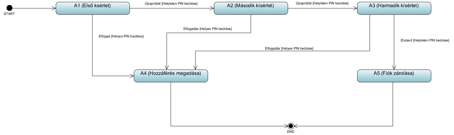
Consider an ATM system function where, if the user enters an invalid PIN three times, the account will be locked. If the PIN is correct on any attempt, the system grants access at that attempt. On the first and second attempts, if the PIN is incorrect, the user receives a warning.

States	Correct PIN entered	Incorrect PIN entered
A1 1st attempt	A4 / Display “Access granted”	A2 / Display Warning #1 (“Incorrect PIN, 2 attempts remaining”)
A2 2nd attempt	A4 / Display “Access granted”	A3 / Display Warning #2 (“Incorrect PIN, 1 attempt remaining”)
A3 3rd attempt	A4 / Display “Access granted”	A5 / Display “Account locked”; disable further input
A4 Access granted	N/A — terminal state	N/A — terminal state
A5 Account locked	A5 / Display “Account locked”; reject input	A5 / Display “Account locked”; reject input

Note: We start from state A0 (START), from which the system automatically enters A1. A4 is a successful terminal state. A5 represents the persistent locked state: further PIN input is rejected and the state remains A5, as shown in TC-05.

State transition diagram for the example:

Test Case Example:

• ID: TC-01
• Objective:Correct PIN entered on the 1st attempt
• Preconditions: A0 → automatically → A1
• Steps: enterPIN(correct)
• Expected State Sequence: A0 → A1 → A4
• Expected outputs: After 1st wrong PIN: Warning #1; 2nd attempt correct → access granted
• Pass Criteria: A4 reached; access granted

Use case testing based on a user story

Use case testing is a black-box test technique that examines the system’s behavior from an actor’s perspective. The tester analyzes use cases and derives tests from their main, alternative, and exceptional flows. The objective is to verify selected end-to-end scenarios and interactions according to the specification; exhaustive coverage of every possible path is rarely feasible.

In an agile development environment, traditional use case documentation is often replaced by the user story, which more concisely expresses the user’s goal and the expected outcome. In this case, use case testing is prepared based on the acceptance criteria associated with the user story: these define what the system must fulfill for the story to be considered “done.” The test cases are therefore directly derived from the user story, covering its main and secondary branches. This approach fits particularly well with collaborative testing, where developers, testers, and business stakeholders jointly identify key examples, behaviors, and exceptions before development begins. As a result, testing truly measures the business goals as interpreted by the user, rather than focusing solely on the technical implementation.

Placing an order from the cart

User story:

As a customer, I want to place an order for the items in my cart, apply a coupon code, and pay by credit card so that I receive confirmation and the goods arrive conveniently.

Acceptance criteria:

1. AC1 – Successful order: Valid cart, valid coupon (if any), successful payment → order ID and email confirmation.
2. AC2 – Invalid coupon: Error message, order can proceed without a coupon.
3. AC3 – Stock change before payment: If any item runs out → error message, order is not finalized.
4. AC4 – Failed payment: Error message, order is not created.
5. AC5 – Incomplete shipping details: Required field indicated; until filled, finalization is not allowed.

Use case (short description):

• Name: Placing an order
• Primary actor: Customer
• Supporting systems: Inventory system, Payment service provider, Email service
• Precondition: The customer has a cart with at least 1 in-stock item; shipping details can be filled in.

Basic (main) flow:

1. Customer opens the “Payment/Checkout” page.
2. System checks inventory for every item.
3. (Optional) Customer enters a coupon code; system validates it.
4. Customer provides/verifies shipping and billing information.
5. Customer selects the payment method and pays.
6. Payment succeeds → the system creates the order, reserves/deducts inventory, sends an email confirmation, and displays the order ID.

Alternative/exception flows:

• A1 (AC2): Coupon invalid → error message, customer decides whether to continue without the coupon.
• E1 (AC3): Out-of-stock during the check → error message, order not finalized, cart updated.
• E2 (AC4): Payment failed/declined → error message, order not created.
• E3 (AC5): Incomplete shipping information → required fields highlighted, submission not allowed.

Test Case Example:

• ID: TC-01
• Source: AC1
• Flow: Main
• Steps: Open cart → Stock OK → Coupon empty → Fill details → Card payment successful
• Expected result: Order ID displayed, email confirmation sent
• Test data: In-stock SKUs

Gherkin code for the test cases:

Feature: Checkout order placement
    In order to receive the products I have selected
    As a customer
    I want to place an order from my cart using an optional coupon and pay by credit card

Background:
    Given I have at least one in-stock item in my shopping cart
    And I am on the Checkout page

@happy_path

Scenario: Successful order without coupon (AC1)
    When I do not enter a coupon code
    And I fill in all shipping and billing information correctly
    And I initiate and approve the credit card payment
    Then the system creates the order and displays the order ID
    And a confirmation email is sent to the customer

@coupon

Scenario: Successful order with a valid coupon (AC1)
    When I enter a valid coupon "SAVE10"
    And I validate the coupon
    And I fill in the shipping and billing details and complete payment successfully
    Then the order is created with the discounted price
    And I receive a confirmation email

@invalid_coupon

Scenario: Handling invalid coupon (AC2)
    When I enter an invalid coupon "BADCODE"
    Then the system displays an error message for the coupon
    When I remove the coupon and complete the payment
    Then the order is created without a coupon
    And a confirmation email is sent

@oos

Scenario: Out-of-stock item before payment (AC3)
    Given one of the items in my cart goes out of stock
    When I attempt to place the order
    Then the system shows an out-of-stock error and does not create the order
    And my cart is refreshed accordingly

@payment_declined

Scenario: Declined payment (AC4)
    When I start the payment and the payment service provider declines the transaction
    Then the system displays an error message and no order is created

@missing_address

Scenario: Missing required shipping information (AC5)
    When I leave the postal code field empty
    And I try to submit the order
    Then the system highlights the required field and prevents order submission

Generating Test Cases with Large Language Models

Large language models can assist with test analysis and test design, but they do not replace a specification, a test strategy, or professional judgement. Their output is a proposal that must be reviewed, traced back to the test basis, and executed where possible.

Artificial intelligence and related concepts

Artificial intelligence (AI) is an umbrella term for computer systems that perform tasks commonly associated with capabilities such as perception, reasoning, learning, language use, planning, or decision support. There is no single universally accepted boundary around the term, so it is useful to distinguish several approaches.

• Rule-based AI uses explicitly programmed knowledge and rules, for example IF condition THEN action. An expert system can explain which rule produced a conclusion, but it does not normally learn new rules from data by itself.
• Classical machine learning (ML) creates a model from examples rather than encoding every decision rule manually. Typical techniques include linear and logistic regression, decision trees, support-vector machines, clustering, and ensemble methods. The learned model is used to predict a value, assign a class, or discover structure in new data.
• Deep learning is a subfield of machine learning based on neural networks with many computational layers. It is especially effective for high-dimensional data such as images, audio, and natural language, but usually requires substantial data and computation.
• Generative AI produces new content—such as text, source code, images, audio, or structured data—based on patterns learned during training. Generative systems do not merely classify an input; they construct an output.
• A large language model (LLM) is a large neural language model trained on extensive text or code data. It represents linguistic patterns in its parameters and can generate or transform sequences of tokens. Most current general-purpose LLMs use the Transformer architecture.

The NIST AI Resource Center glossary and the Google Machine Learning Glossary provide broader collections of AI terminology.

Language models and LLMs

A language model assigns probabilities to sequences of tokens. An autoregressive language model generates text step by step: based on the preceding tokens, it estimates a probability distribution for the next token, selects or samples one token according to the decoding settings, appends it to the context, and repeats the process.

It is therefore only approximately correct to say that an LLM “returns the statistically most likely answer.” The model estimates likely tokens, not the truth of complete statements. With greedy decoding it may select the highest-probability next token; with sampling, temperature, or other decoding strategies it may deliberately select a less probable token. In neither case does probability imply factual correctness.

What is the temperature?

Temperature is a parameter that controls how an LLM selects the next token from its predicted probability distribution.

• Low temperature makes the output more deterministic and conservative. Tokens with the highest predicted probabilities are strongly preferred.
• High temperature makes the probability distribution flatter. Less probable tokens are selected more often, producing more varied but also less predictable output.

An LLM does not, by default, independently verify every statement it generates. It may produce an answer that is grammatically convincing but unsupported, inconsistent, incomplete, or factually incorrect. In generative-AI terminology, such unsupported content is often called a hallucination or confabulation.

An agentic AI system can place an LLM in a control loop in which it plans steps, invokes tools, observes their results, and revises its work. For example, an agent may retrieve a requirement from a controlled repository, execute generated tests, inspect failures, or check a factual statement against an authoritative source. This can improve reliability, but it does not guarantee correctness: the agent may choose the wrong source, misuse a tool, misinterpret a result, or stop too early. Tool outputs, permissions, termination criteria, and human review therefore remain important.

Tokenization

An LLM does not normally process text as whole words. A tokenizer converts text into tokens and maps each token to an integer identifier. A token may represent a complete word, a word fragment, punctuation, whitespace, or a byte sequence. Consequently, token boundaries depend on the tokenizer and language: one word may consist of one token in one context and several tokens in another. Context limits and usage costs are generally measured in tokens rather than characters or words.

Embeddings

An embedding is a learned numerical vector representation of an item such as a token, sentence, document, image, or source-code fragment. Items used in similar contexts often receive vectors that are close according to a selected similarity measure. Inside an LLM, token embeddings are part of the model’s computation. Separate embedding models are also used for semantic search and retrieval-augmented generation. Similarity in an embedding space expresses learned statistical relatedness; it is not, by itself, a formal proof that two items have the same meaning.

Uses of LLMs in software testing

An LLM can assist throughout the testing process:

• Requirement analysis: identify actors, conditions, actions, boundaries, contradictions, missing cases, undefined terms, and requirements that are difficult to test.
• Test-condition identification: propose functional, non-functional, positive, negative, boundary, robustness, security, and error-handling conditions.
• Test-case generation: derive candidate test cases using equivalence partitioning, boundary value analysis, decision tables, state transitions, use cases, pairwise combinations, or risk-based selection.
• Test-oracle support: propose expected results from an explicit specification or an executable reference model.
• Test automation: generate test code, fixtures, mocks, stubs, page objects, API requests, database setup, assertions, and CI configuration.
• Test-data generation: produce valid, invalid, boundary, synthetic, or privacy-preserving sample data.
• Result analysis: summarize logs, cluster similar failures, compare expected and actual results, and suggest possible causes for investigation.
• Testware production: draft test plans, traceability matrices, test reports, defect reports, checklists, and supporting documentation.
• Maintenance: update candidate tests and documentation when requirements or interfaces change.

Testware

Testware comprises the work products created or used during testing. Depending on the project, it may include test plans, test conditions, test cases, test procedures, test scripts, test data, test environments, stubs, drivers, expected results, execution logs, defect reports, coverage reports, and test-summary reports. Testware includes more than executable test code. The term is also defined in the ISTQB glossary.

An LLM is not an authoritative test oracle

A test oracle is a source used to determine the expected result of a test. An LLM may help interpret a requirement or formulate an expected result, but its own generated answer is not sufficient evidence that the expected result is correct. Whenever possible, expected results should be grounded in an approved specification, formal rule, trusted reference implementation, independently calculated value, domain expert decision, or another controlled source.

Prompts and prompt engineering

A prompt is the input supplied to a generative model. It may contain instructions, questions, examples, source material, data, constraints, and a required output format. In conversational systems, the effective prompt may also include earlier messages and system-level instructions that are not visible in the latest user message.

Prompt engineering is the iterative design and evaluation of prompts so that the model produces outputs that are more relevant, consistent, testable, and suitable for a particular task. It is not a method for proving correctness. A good prompt reduces ambiguity and makes omissions easier to detect, but the resulting output must still be evaluated. The OpenAI prompt-engineering guide presents additional practical patterns.

A practical prompt framework contains the following elements:

Element	Purpose	Example
Role	Defines the perspective or expertise to apply	“Act as a senior software test analyst.”
Context	Describes the system, domain, and objective	“We are testing a residential energy controller.”
Instruction	States the task to perform	“Derive test conditions and a decision table.”
Input	Supplies the authoritative source material	Requirements, user stories, API specification, source code
Constraints	Limits assumptions and defines rules	“Do not invent missing business rules; list ambiguities.”
Output format	Makes the result inspectable and reusable	Markdown tables with IDs and traceability

The order is flexible. What matters is that the model can distinguish authoritative input from instructions and that missing information is not silently replaced by invented assumptions.

Reusable prompt for test-case generation

Role:
Act as a senior software test analyst experienced in black-box test design.

Context:
The supplied text is the complete test basis for a system feature.
The output will be reviewed by a human tester before use.

Instruction:
1. Extract atomic requirements and assign IDs R1, R2, ... .
2. List contradictions, ambiguities, and missing rules. Do not resolve them silently.
3. Identify valid and invalid equivalence partitions and boundary values.
4. Create a minimized decision table containing all feasible business-rule combinations.
5. Derive a minimal test set from the table and add important negative and boundary tests.
6. Check every test against the supplied requirements before returning it.

Input:
<paste the specification here>

Constraints:
- Use only information in the input.
- Clearly label every assumption.
- Do not treat generated expected results as verified facts.
- Do not include infeasible combinations as executable test cases.
- Keep condition values and expected actions separate.

Output format:
A. Atomic requirements
B. Questions and ambiguities
C. Equivalence partitions and boundaries
D. Decision table
E. Test cases with columns:
   ID | Source requirement/rule | Preconditions | Input | Expected result
F. Coverage and limitations

A controlled workflow for LLM-assisted test generation

1. Prepare the test basis. Remove irrelevant content, identify authoritative sources, and exclude secrets and personal data.
2. Ask for analysis before generation. Require the model to extract rules and list ambiguities before it creates tests.
3. Choose an explicit technique. For example, request a decision table rather than merely asking for “all tests.”
4. Require traceability. Every generated test should refer to a requirement, rule, state transition, risk, or coverage item.
5. Review expected results independently. Pay particular attention to calculations, precedence rules, units, dates, and legal or domain-specific decisions.
6. Generate automation only after reviewing the abstract tests. Otherwise, a misunderstanding can be reproduced consistently in many lines of plausible-looking code.
7. Compile and execute generated code. Static inspection alone is insufficient. Review dependencies, assertions, cleanup behavior, nondeterminism, and security consequences.
8. Measure usefulness. Track accepted, modified, rejected, duplicate, invalid, and defect-revealing generated tests. A large number of generated tests is not evidence of good coverage.
9. Preserve provenance. Store the model, prompt, input version, generation date, output, reviewer, and subsequent modifications when reproducibility or auditability matters.

Typical failure modes include invented requirements, incorrect expected results, missing boundary cases, duplicate tests, infeasible combinations, assertions that merely repeat the implementation, brittle selectors, invalid API calls, fabricated library functions, and disclosure of confidential data through prompts.

Exercises

Residental Energy System

A house is equipped with solar generation, a wind turbine, and battery storage. The controller must coordinate energy-source selection, storage, household supply, and feed-in to the grid.

• If solar or wind energy is available and the battery is not full, the battery is charged from renewable energy.
• If renewable energy is unavailable, controlled-tariff electricity may be used to charge the battery when it is available.
• Charging must stop when the battery reaches 100%.
• If the battery is full and renewable energy is available, the renewable energy is fed into the grid.
• Household consumption is supplied from the battery while stored energy is available. Charging and discharging may occur simultaneously from the controller’s perspective.
• If the battery is empty, the house is supplied from the ordinary grid.
• The ordinary grid must never charge the battery.
• Stored battery energy must never be fed into the grid.

Prompt for the residential energy controller

Role: Act as a senior test analyst.

Context: We are testing the control logic of a residential energy system.

Instruction:
Analyze the requirements below. First list ambiguities and missing precedence
rules. Then create minimized decision tables for (1) battery charging and
renewable feed-in and (2) the source of household consumption. Derive test
cases from every rule and add boundary tests for 0% and 100% state of charge.

Input:
<paste the residential energy-controller requirements here>

Constraints:
Do not invent power limits, efficiency values, timing behavior, or a priority
between solar and wind generation. Treat solar OR wind as “renewable available”.
A dash in the decision table means “irrelevant”. Keep ordinary-grid supply and
controlled-tariff charging separate. Never permit ordinary-grid charging or
battery-to-grid feed-in.

Output format:
  1. Requirement questions
  2. Decision tables
  3. Test cases with traceability

The specification leaves several questions unanswered: What happens when solar and wind energy are available simultaneously? Is their production aggregated? What exact threshold represents an empty battery? Can controlled-tariff electricity supply the house directly? What happens when renewable production is smaller than household demand? How are maximum charge and feed-in powers handled? These questions should be resolved before quantitative or timing tests are designed.

For the stated Boolean control rules, renewable availability can be defined as R = solar_available OR wind_available.

Conditions and actions	E1	E2	E3	E4	E5
Renewable energy available (R)	T	T	F	F	F
Controlled-tariff electricity available (C)	–	–	T	F	–
Battery full (F)	F	T	F	F	T
Charge from renewable energy	X
Charge from controlled-tariff electricity			X
Feed renewable energy into grid		X
Do not charge or feed in				X	X

Conditions and actions	H1	H2
Battery empty	F	T
Supply house from battery	X
Supply house from ordinary grid		X

These two tables are intentionally separated because the specification permits charging and discharging at the same time. Tests may combine one rule from each table when interaction coverage is required.

Test Case Example:

• ID: EC-01
• Rules: E1+H1
• Preconditions/input: Renewable available; battery at 50%; battery not empty
• Expected result: Charge from renewable energy while supplying the house from the battery

Policyholder reward

An insurance association plans to enter the stock market and offer a reward to members for their previous customers. A current policyholder is eligible only if the policy carries dividend rights. A qualifying policyholder who has owned the policy since 2001 may choose between cash and shares in the new company. A qualifying policyholder who has held the policy for a shorter period is eligible for cash only. When the share allocation is calculated, the number of customers is weighted as follows:

• fewer than 10 customers: multiplier 1;
• 10–19 customers: multiplier 2;
• 20–49 customers: multiplier 3;
• 50 or more customers: multiplier 5.

Prompt for the policyholder reward

Role: Act as a senior test analyst specializing in decision-table testing.

Context:
We are testing a policyholder reward calculation for an insurance association.

Instruction:
Convert the supplied reward rules into atomic requirements. Identify ambiguous
eligibility and date-boundary rules. Create a minimized mixed-entry decision
table, then derive tests for every rule and every
customer-count boundary.

Constraints:
Do not assume that “since 2001” means a specific date until it is clarified.
Distinguish “no reward”, “cash only”, and “choice of cash or shares”. Apply a
share multiplier only when shares may be selected. Use “–” for irrelevant
conditions and do not invent a multiplier of 4.

Input:
<paste the policyholder-reward requirements here>

Output format:
A. Questions
B. Decision table
C. Test cases with source-rule references

Important questions include whether “since 2001” means continuously since 1 January 2001, acquired at any time during 2001, or owned for a fixed number of years; whether former policyholders are excluded; and whether exactly 0 customers is valid. The following table uses the abstract condition ownership-duration requirement met so that it does not silently choose a date interpretation.

Conditions and actions	P1	P2	P3	P4	P5	P6	P7
Current policyholder	F	T	T	T	T	T	T
Dividend-entitling policy	–	F	T	T	T	T	T
Ownership-duration requirement met	–	–	F	T	T	T	T
Customer-count band	–	–	–	<10	10–19	20–49	≥50
No reward	X	X
Cash only			X
Choice of cash or shares				X	X	X	X
Share multiplier	–	–	–	1	2	3	5

Test cases:

Test ID	Rule	Input	Expected result
PR-01	P1	Former policyholder; otherwise qualifying data	No reward
PR-02	P2	Current policyholder; policy has no dividend rights	No reward
PR-03	P3	Current qualifying policy; duration requirement not met	Cash only; shares unavailable
PR-04	P4	Eligible for choice; 9 customers	Cash or shares; share multiplier 1
PR-05	P5	Eligible for choice; 10 customers	Cash or shares; share multiplier 2
PR-06	P5	Eligible for choice; 19 customers	Cash or shares; share multiplier 2
PR-07	P6	Eligible for choice; 20 customers	Cash or shares; share multiplier 3
PR-08	P6	Eligible for choice; 49 customers	Cash or shares; share multiplier 3
PR-09	P7	Eligible for choice; 50 customers	Cash or shares; share multiplier 5

The boundary values 9/10, 19/20, and 49/50 are essential. Tests should also cover 0, negative, non-integer, missing, and extremely large customer counts according to the input contract. Until that contract is specified, the expected handling of invalid counts must remain an open question rather than an invented result.

Neptun course enrollment

Design the acceptance tests of the course enrollment function based on user story + acceptance criteria, using a black-box approach.

Background (short domain):

Course enrollment is only successful if:

• the student has met all prerequisites, and
• the course is open for enrollment (capacity not full).

Success: enrollment confirmation.

Failure: the system provides an appropriate message (“Prerequisite not met” or “Course is full”) and offers:

• finishing the operation, or
• searching for another course.

The student can search among courses (by code, name, instructor, time).

US1 – Course enrollment: As a student, I want to enroll in the selected course so that I can progress in my studies.

US2 – Error handling and suggestion: As a student, I want to receive a clear message on failed enrollment and be offered to finish or search again so that I can quickly find an alternative.

US3 – Course search: As a student, I want to search for courses by multiple criteria so that I can find the one that suits me.

Acceptance criteria (short):

• AC1 – Successful enrollment: If all prerequisites are met and there is free capacity, the system records the enrollment and confirms it.
• AC2 – Missing prerequisite: If any prerequisite is missing, the system reports this and offers: Finish | Search for another course.
• AC3 – Full capacity: If there is no free capacity, the system reports this and offers: Finish | Search for another course.
• AC4 – Search operation: Filter courses by code/name/instructor/time; result list is sortable.
• AC5 – Display of branching options: For every failure, the two options (finish/search) are shown.
• AC6 – Race condition (optional, bonus): If capacity runs out at the last moment, correct error and offer per AC3.

Create test cases based on US1–US3 and AC1–AC6! Use a use case testing approach: main flow, alternatives, exceptions.

Railway signalling system

A railway colour-light signal is to be tested.

• The signal controls entry, from the direction of the signal, into the track section behind it.
• The protected section extends to the next signal and contains no junction. A train can therefore enter or leave it only at one of its two ends.
• A detector at each end indicates when a train is entering or leaving the section at that end.
• The signal is notified when the next signal changes between a restrictive and a permissive state. It can similarly report changes in its own permissive or restrictive state to the preceding signal.
• Rail traffic on the section is bidirectional. Among other safety functions, the signalling system must prevent simultaneous use in opposing directions.
• The signal can display STOP, PROCEED WITH CAUTION, or PROCEED.
• If a train occupies the protected section, the signal must display STOP. If the section is unoccupied but the next signal is restrictive, the signal must display PROCEED WITH CAUTION. Otherwise, it must display PROCEED.
• The system must detect inconsistent states and emergencies. In either case, it must change to STOP and notify the control centre. Recovery is possible only through a manual physical intervention or restart, which is outside normal operation.

Testing the railway signalling system

Use a state-transition diagram to derive test cases for the system.

One possible solution

The following model is one possible abstraction. It assumes that the detector interface has already interpreted the two endpoint signals as TRAIN_ENTERED or TRAIN_LEFT relative to the protected section. A real interlocking system would also retain the detector identity, travel direction, axle count or another train-integrity indication, and direction-locking information.

Input events

• TRAIN_ENTERED: a train enters the protected section at either end;
• TRAIN_LEFT: a train leaves the protected section at either end;
• NEXT_CHANGED_TO_RESTRICTIVE: the next signal changes to a restrictive state;
• NEXT_CHANGED_TO_PERMISSIVE: the next signal changes to a permissive state.

Outputs

• LIGHT_STOP, LIGHT_CAUTION, or LIGHT_PROCEED changes the displayed aspect;
• PASSAGE_BLOCKED or PASSAGE_PERMITTED reports the local restrictive/permissive state to the preceding signal;
• FAULT reports an inconsistent event or state to the control centre;
• EMERGENCY reports an unsafe event, such as a second entry into an occupied section.

States

• S1 — clear and unoccupied: the section is empty, the next signal is permissive, and the local signal displays PROCEED.
• S2 — occupied, next signal permissive: the protected section is occupied, so the local signal displays STOP.
• S3 — unoccupied, next signal restrictive: the section is empty, and the local signal displays PROCEED WITH CAUTION.
• S4 — occupied, next signal restrictive: the protected section is occupied, so the local signal displays STOP.
• S5 — latched fault or emergency: the local signal displays STOP, passage is blocked, and normal events cannot restore operation.

State transitions

stateDiagram-v2
    [*] --> S1
    S1 --> S2: TRAIN_ENTERED / STOP
    S1 --> S3: NEXT_RESTRICTIVE / CAUTION
    S2 --> S1: TRAIN_LEFT / PROCEED
    S2 --> S4: NEXT_RESTRICTIVE
    S3 --> S4: TRAIN_ENTERED / STOP
    S3 --> S1: NEXT_PERMISSIVE / PROCEED
    S4 --> S3: TRAIN_LEFT / CAUTION
    S4 --> S2: NEXT_PERMISSIVE
    S1 --> S5: inconsistent / FAULT
    S2 --> S5: inconsistent or second entry
    S3 --> S5: inconsistent / FAULT
    S4 --> S5: inconsistent or second entry
    S5 --> S5: any normal event / remain STOP

Derived tests

1. Execute every valid transition shown above at least once and verify both the destination state and every specified output.
2. In each unoccupied state, issue TRAIN_LEFT; verify transition to S5, the STOP aspect, blocked passage, and a FAULT notification.
3. In each occupied state, issue another TRAIN_ENTERED; verify transition to S5, the STOP aspect, blocked passage, and an EMERGENCY notification.
4. In each state, issue a notification that claims the next signal has changed to the value already represented by that state. Under the stated change-event contract, verify that this is detected as inconsistent and latched in S5.
5. Reach S5 through every defined fault and emergency path. Then apply each normal event in turn and verify that none of them releases the latched state.
6. Exercise the transition pairs S1 → S2 → S4 → S3 → S1 and S1 → S3 → S4 → S2 → S1 to cover changes of the next signal both before and during occupancy.
7. For bidirectional operation, repeat entry and exit tests using both endpoint detectors. Verify that the occupied state blocks a second entry from either end, including an entry in the opposing direction.

The original simplified transition table requires two corrections. When the next signal becomes permissive in S4, the correct destination is S2, not S3, because the section remains occupied. In addition, the transitions S1 → S3 and S3 → S1 must change the displayed aspect to PROCEED WITH CAUTION and PROCEED, respectively.

Billing System

A telecommunications company is developing billing software. The charge calculation is fairly complex, and several types of discounts are available. The base rate is 1 petak per second. During peak hours—between 08:00 and 16:00 every day—the rate is 150% of the base rate. At night—between 22:00 and 06:00 every day—the rate is 75% of the base rate. As a commercial discount, calls made within the same network are always 40% cheaper. Age-based discounts are also available: customers under 18 receive a 10% discount, while children under 14 receive an additional 10% discount. Customers between the ages of 18 and 26 receive a 5% discount. For calls lasting longer than 15 minutes, a 15% discount applies to the portion exceeding 15 minutes. Calls lasting longer than 30 minutes receive a 30% discount. Discounts granted on different grounds are additive. Calls between phones belonging to the same fleet are free outside peak hours. International calls, however, are always charged at a rate of 3 petaks per second.

Identify the individual test elements. Assign test cases to each test element using several different test-design techniques.

Solution

• Equivalence Partitioning (EP):
  • Time period: { Night, Off-peak, Peak } or { [00:00:00–05:59:59], [06:00:00–07:59:59], [08:00:00–15:59:59], [16:00:00–21:59:59], [22:00:00–23:59:59] }
  • Duration: { Short = [00:01–15:00], Medium = [15:01–30:00], Long = [30:01 or longer] }
  • Age: { Child = under 14, Minor = 14–17, Young adult = 18–25, Adult = 26 or older }
  • Destination: { Fleet, Same network, Domestic, International }
• Boundary Value Analysis (BVA):
  • Time period:
    • Two-point BVA: 00:00:00, 05:59:59, 06:00:00, 07:59:59, 08:00:00, 15:59:59, 16:00:00, 21:59:59, 22:00:00, 23:59:59
    • Additional values for three-point BVA: 00:00:01, 05:59:58, 06:00:01, 07:59:58, 08:00:01, 15:59:58, 16:00:01, 21:59:58, 22:00:01, 23:59:58
  • Duration:
    • Two-point BVA: 00:00, 00:01, 15:00, 15:01, 30:00, 30:01
    • Additional values for three-point BVA: 00:02, 14:59, 15:02, 29:59, 30:02
  • Age measured in completed years:
    • Two-point BVA: 13, 14, 17, 18, 25, and 26 years
    • Additional values for three-point BVA: 12, 15, 16, 19, 24, and 27 years
  • Age calculated with day-level precision:
    • Two-point BVA: one day before the 14th birthday, the 14th birthday, one day before the 18th birthday, the 18th birthday, one day before the 26th birthday, and the 26th birthday
    • Additional values for three-point BVA: two days before the 14th birthday, one day after the 14th birthday, two days before the 18th birthday, one day after the 18th birthday, two days before the 26th birthday, and two days after the 26th birthday
• • Minimal each-value coverage: 4 test cases: 1, 70, 139, and 48
  • Pairwise coverage: 16 test cases: 1, 13, 24, 27, 38, 55, 64, 66, 78, 89, 92, 100, 106, 117, 131, and 143
  • Exhaustive coverage: 144 test cases: 1–144

  Combination testing — after applying decision-table testing:

  Some test cases:

  TC	1	2		48	49		70		96	97		139		144
  Time Period	N	N		N	O-P		O-P		O-P	P		P		P
  Duration	S	S		L	S		M		L	S		L		L
  Age	C	C		A	C		Y		A	C		O		A
  Destination	F	S		I	F		S		I	F		D		I

---

Utolsó frissítés: 2026-09-04 08:34:02